Overview
Regardless of the application, calculating a particular statistic and associated p-value is not necessarily the biggest challenge in designing experiments. Indeed, given the availability of open source software packages such as scipy and statsmodels in Python, calculating a test statistic is simple and easy. Instead, ensuring that the assumptions required for a statistical test are actually satisfied by the data is far more challenging. Most real world data — in addition to being dirty — will not satisfy these assumptions without careful thinking about experimental design. For example, many test statistics require that the observations or measurements in the data be independent and identically distributed. Furthermore, for parameterized statistical tests, the data also must follow a particular distribution described by the test parameters. Thankfully, because of the Central Limit Theorem, a normal distribution approximates the distribution of many test statistics with a sufficiently large sample size, and thus textbook statistical tests such as the t-test or Z-test can be used. Even then, a data analyst or data scientist must carefully validate that appropriate sampling techniques are used to avoid inappropriate or misleading business and scientific recommendations based on invalid experiments.
In this blog post, I discuss independence, sampling, and experimental design in the context of my work as a data scientist at Synthego, a biotech manufacturing company. I use a simulated, clean, and simplified data set with features similar to our manufacturing data to demonstrate fundamental statistical concepts and challenges in experimental design. Although the context is chemistry and manufacturing, the core concepts are highly relevant in other contexts, such as designing an A/B testing framework.
The data used in this blog post and the associated code are available via Github.
Introduction
Background
Synthego produces chemically modified synthetic guide RNA as a major product for use with the gene editing technology CRISPR-Cas9. Customers order unique RNA sequences that correspond to the target DNA sequence they want to edit. Ninty-six custom sequences are synthesized simultaneously on a 96-well plate shown schematically below:
   1  2  3  4  5  6  7  8  9 10 11 12
  ___________________________________
A|00|01|02|03|04|05|06|07|08|09|10|11|
B|12|13|14|15|16|17|18|19|20|21|22|23|
C|24|25|26|27|28|29|30|31|32|33|34|35|
D|36|37|38|39|40|41|42|43|44|45|46|47|
E|48|49|50|51|52|53|54|55|56|57|58|59|
F|60|61|62|63|64|65|66|67|68|69|70|71|
G|72|73|74|75|76|77|78|79|80|81|82|83|
H|84|85|86|87|88|89|90|91|92|93|94|95|
  –––––––––––––––––––––––––––––––––––
where the 8 rows correspond to the letters A through H, and the 12 columns correspond to the integers 1 through 12. Each well also has an integer index from 0 to 95 starting from left to right and top to bottom. After synthesis, the entire plate undergoes simultaneous post-processing and purfication steps, and the purity and amount of material is measured. If a well has insufficient RNA material to meet the customer order or contains too many impurities, the associated sequence is re-synthesized. As such, ensuring that enough pure material is synthesized and purified is crucial to ship orders on time at low cost.
Data definitions
Synthetic (see what I did there), simplified, and clean data was randomly generated for the purposes of this blog post. Keep in mind that the real data from Synthego's manufacturing process (or from anything else for that matter) will not nearly be as clean or have as clear behavior as this. One thousand syntheses with 96 wells each were simulated to create a 96,000 row data set. The data contains several fields describing the amount and purity of the material and synthesis metadata. In the actual manufacturing process, impurities are measured with mass spectrometry and an algorithm that fits known and unknown impurity mass peaks in a spectrum. Common impurities include sequences with one extra or missing nucleotide (base) or with poor purification or post-processing.
Metadata
synthesis_id: integer identifier for a synthesiswell_position: integer identifier for a wellwell_position_label: position label for a well on a 96-well plate (letters for rows and numbers for columns)
Pure product metrics
pure_yield: amount of pure material after synthesis and purification in nanomoles (nmol)full_length_product: percent of full length product
Impurity metrics
n-1: percent of material missing one nucleotiden+1: percent of material with one extra nucleotidecyanoethyl: percent of material with an impurity associated with a particular bad reagentother_impurity: A non-specific measure of impurities not directly fit (a ratio from 0 to 1)
Data Exploration
Well-level data
Of course, before we dive too much into anything, we need to explore the data! (Pro-tip: Always. Do. EDA. On. Unknown. Data.) First, we want to look at the distribution of each of our six metrics. The plotting library seaborn has a useful method here called distplot that combines a histogram with kernel density estimation (KDE) to provide a good sense of the distribution of a metric. We can also fit a distribution function from scipy to this distribution. The actual plot for pure yield and the Python code to generate it is shown below:
import pandas as pd
import matplotlib.pyplot as plt
import seaborn as sns

df = pd.read_csv('synthetic_data.csv')

fig, ax = plt.subplots(figsize=(5, 5))
sns.distplot(df['pure_yield'], fit=scipy.stats.distributions.norm)
ax.set_xlabel('Pure Yield (nmol)', fontsize=14)
ax.set_ylabel('Density', fontsize=14)
plt.show()
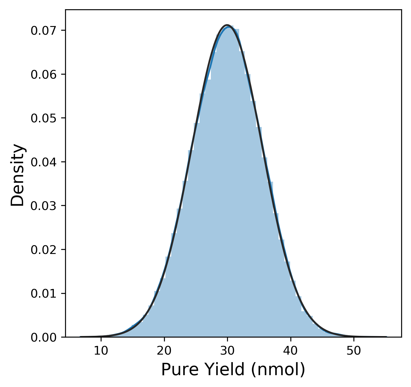
The distribution for the pure yield is pretty clearly normally distributed from this plot (The fit to the normal distribution almost entirely overlaps with the KDE plot.)
We can use this same code snippet (rewritten as a function in the code on Github) to generate distribution plots for each of our metrics described above:
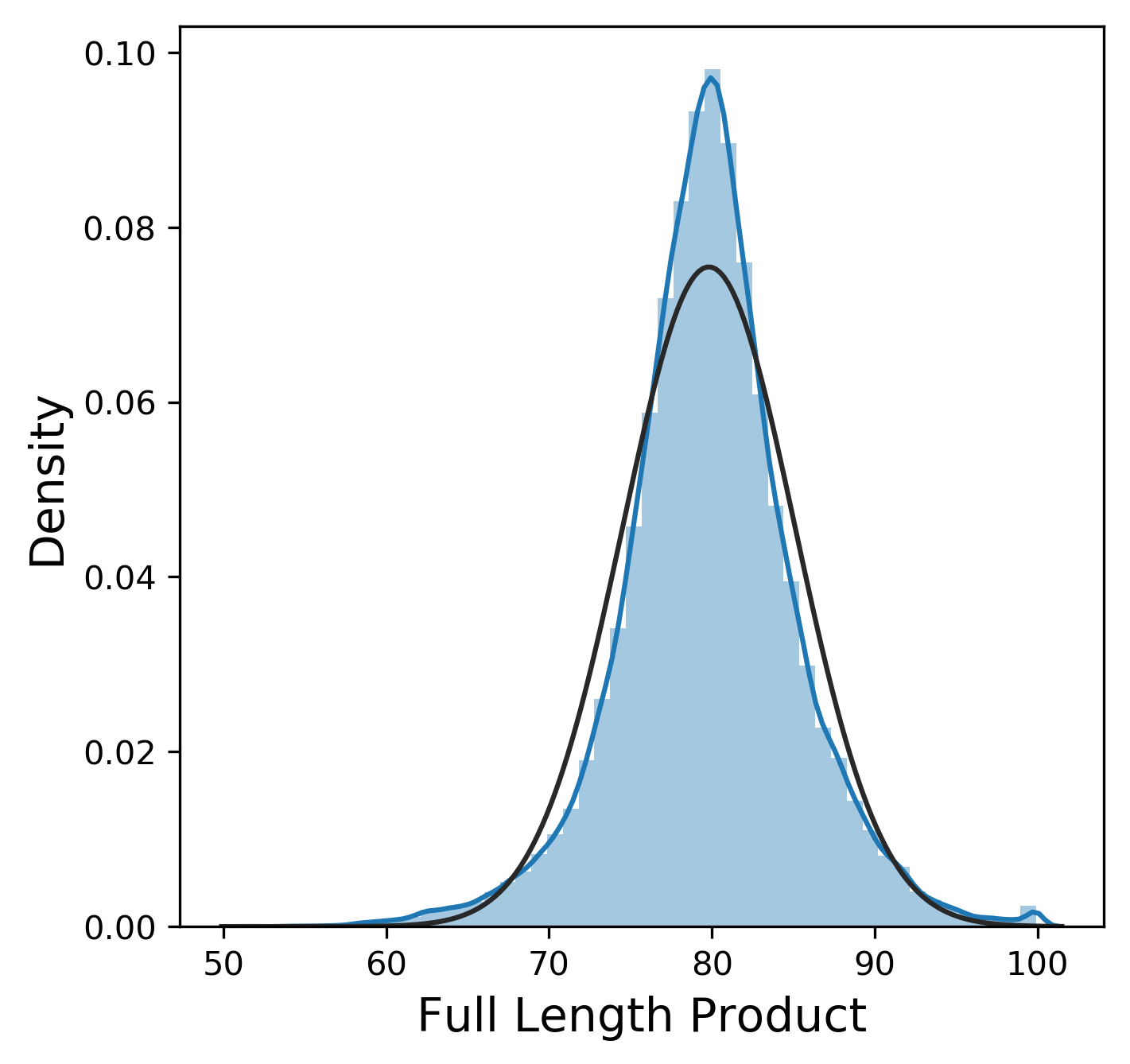
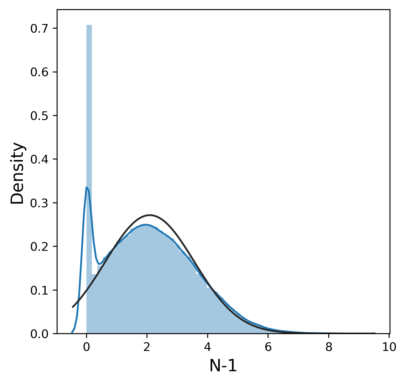
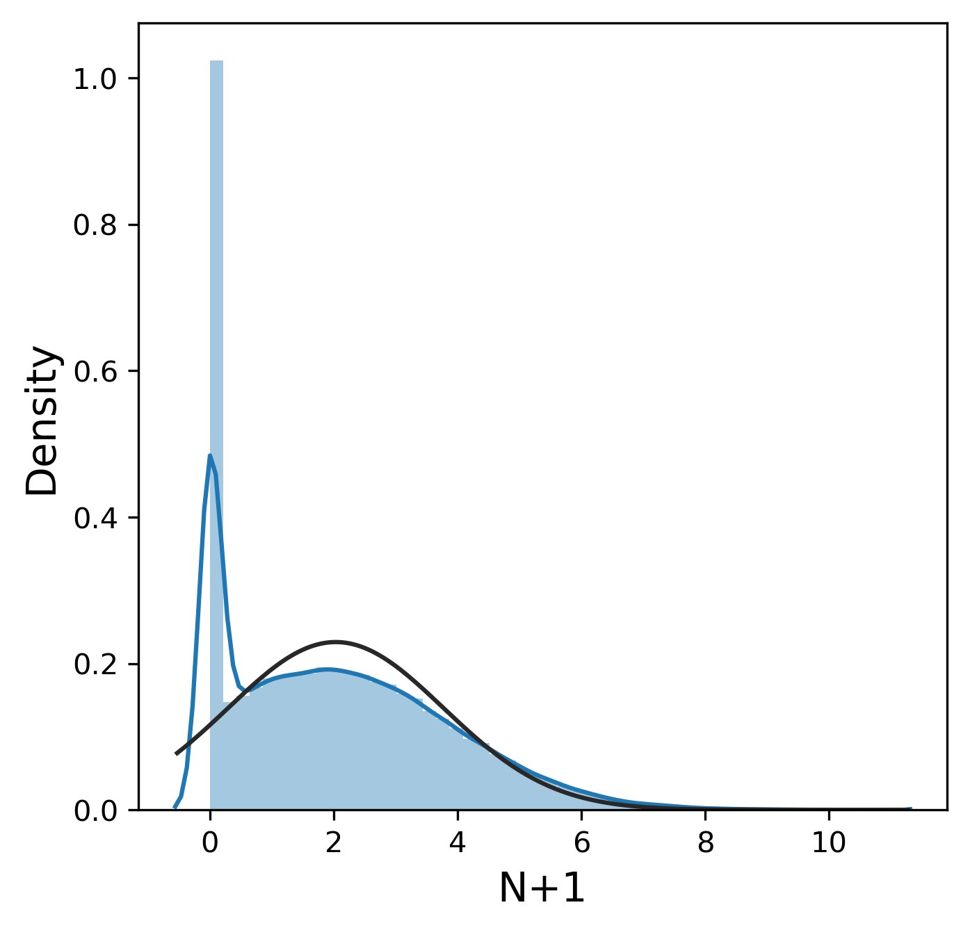
Much like the pure yield, most of these metrics have a mostly normal distribution, although sometimes we were lucky enough to get 99.9% pure product and thus 0% n-1 and n+1. In contrast, other_impurity has a distinctly non-normal distribution, where most of the values cluster near 0 with a few extreme values near 1. This is clearly an unusual distribution compared to the rest of the metrics, but we will ignore this for now.
To get a sense for how the different metrics might be interrelated (if at all), we can also plot the correlation between the various metrics as a heatmap.
We can see that most metrics are not actually correlated at all, except negative correlations n-1 and n+1 with full_length_product, and a mild positive correlation between n-1 and n+1. Clearly, if we have a poor synthesis (many additions and deletions), we will get less of our desired material. The other metrics (cyanoethyl and other impurity) are more related to post-processing and not necessarily strongly related to the other metrics.
Synthesis-level data
Looking at the overall population of wells is certainly important, but what about individual syntheses? We might assume each synthesis is a random sample of 96 individual wells, but that might not actually be the case. Since each RNA guide in the wells on a plate are produced simultaneously, we might see similar effects on the same plate for various reasons (e.g., a bad reagent bottle, accidentally exposing the whole plate to air or water, some hardware failure on the synthesizer, etc.) To examine the behavior of syntheses, we can summarize the data by synthesis using groupby in pandas using this common coding pattern:
# Initialize list
results = []

for synthesis_id, group in df.groupby('synthesis_id'):

    # Create dictionary record of summary metrics, and append to results
    data = {
        'synthesis_id': synthesis_id,
        'pure_yield': group.pure_yield.mean(),
        'full_length_product': group.full_length_product.mean(),
        # etc.
    }

    results.append(data)

# Convert list of records into pandas DataFrame
synthesis_df = pd.DataFrame(results)
Now we have a new data frame of length 1000 that summarizes each of the syntheses in our original data set. We could also look at other summary statistics besides the mean here, but for now let's focus on the behavior the synthesis means. Shown below is a plot comparing the distribution of the pure yields on each well to the distribution of the mean pure yield on each synthesis (with only the KDE of each distribution shown for clarity.)
Here, the distribution of the synthesis mean of the pure yield is a bit narrower than the distribution of the pure yield on each well, but not by much. How does this compare to a random sample of 96 wells? Instead of grouping by synthesis, we could take 1000 random samples of 96 wells from all wells, calculate the mean, and compare the distributions.
results = []
for _ in range(1000):
    sample = df.sample(n=96)

    data = {
        'pure_yield': sample['pure_yield'].mean(),
        'full_length_product': sample['full_length_product'].mean(),
        # etc.
    }

    results.append(data)

resampled_df = pd.DataFrame(results)
Once we've generated these samples, we can then plot the distribution of the sample pure yield means with the distributions for the wells and synthesis means.
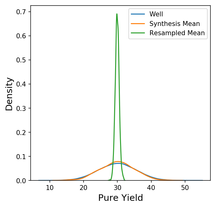
Why do we see a much narrower distribution for a random sample of 96 wells versus the 96 wells on a synthesis? For that, we turn to the Central Limit Theorem.
Experimental Design, Sampling, and the Central Limit Theorem
Central Limit Theorem
The Central Limit Thoerem, one of the most important theorems in statistics and probability, describes what to expect mathematically when we randomly sample from a population of an independent, identically distributed parameter with mean \(\mu\) and standard deviation \(\sigma\). Namely, if we generate random samples of this parameter of size n, the sample mean \(\bar{x}\) will approximate a normal distribution with mean \(\mu\) and standard deviation \(\sigma / \sqrt{n}\) as \(n\) increases.
Therefore, a random sample of 96 wells should have a standard deviation equal to the population standard deviation divided by the square root of 96. Let's compare the standard deviation for the entire population of wells, synthesis means, random sample means, and predictions of the Central Limit Theorem.
| Group | Mean | Standard Deviation |
|---|---|---|
| Well (Population) | 29.953 | 5.605 |
| Synthesis | 29.953 | 5.025 |
| Random Sample | 29.944 | 0.582 |
| Predicted | 29.953 | 0.572 |
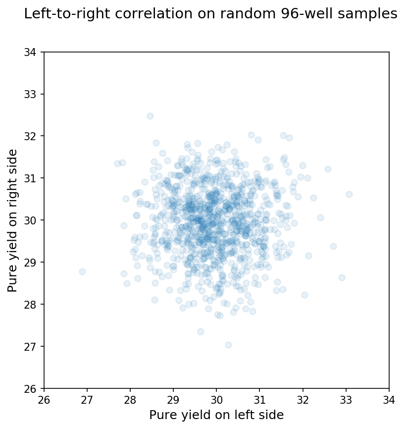
Clearly, the random sample matches our predictions from the Central Limit Theorem, and the 96 wells on an individual synthesis are not random samples from the larger population of wells. We can see this another way by comparing the means between arbitrary subsets of a synthesis or random sample. In this case, I just compared the mean for wells on the left half of the 96-well plate to the mean for wells on the right half of the 96-well plate for a synthesis or random sample. For 96-well random samples, we see almost no correlation between the means from each side as shown below:
In contrast, when we compare the means on the left side of the plate with those for the right side of the same synthesis, we see a pretty clear relationship as shown below:
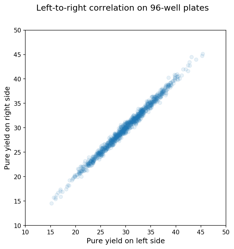
Thus, the wells on a synthesis are not independent units but are actually interdependent for the reasons mentioned above (e.g., a bad reagent bottle affects the whole synthesis, etc.)
Experimental Design Consequences
OK, so what? Sure, the Central Limit Theorem, sampling, independence, and all that are interesting in an abstract sense, but how does this help design better experiments? Well, if we're not careful about randomization in our experimental design, we could end up with spurious results!

One unfortunately common type of bad experimental design. (Credit: XKCD)
For example, let's suppose we are testing whether some new process change has a positive effect on pure yield. Our null and alternative hypotheses would then be the following:
\(H_0: \text{pure yield}_{\text{new}} = \text{pure yield}_{\text{old}}\)
\(H_a: \text{pure yield}_{\text{new}} > \text{pure yield}_{\text{old}}\)
We then run a single control synthesis with our old process and a single treatment synthesis with our new process and get the following results:
| Synthesis ID | Experimental Group | Mean | Standard Deviation |
|---|---|---|---|
| 3 | Control | 26.431 | 2.331 |
| 4 | Treatment | 36.597 | 2.590 |
Looks promising, right? We then naively assume that each well is independent and that a synthesis is a random sample of 96 wells. We perform a t-test with our experimental results and those assumptions as shown below:
import scipy

control_mask = df.synthesis_id == 3
treatment_mask = df.synthesis_id == 4

t_test_results = scipy.stats.ttest_ind(df.loc[treatment_mask, 'pure_yield'],
                                       df.loc[control_mask, 'pure_yield'])
print(t_test_results)
# Output: Ttest_indResult(statistic=28.581, pvalue=1.014e-70)
Whoa, our t-statistic is 28.6 with a p-value of \(1 \times 10^{-70}\); we should definitely reject the null hypothesis. Clearly, our new process change is amazing, and we're super geniuses for thinking of it. Is that really true, though?
Unfortunately, one of the key assumptions of the t test is that the samples have been randomly drawn from the larger population. As we discussed earlier, a synthesis is not a random sample of 96 wells, though! So, our new process change might be amazing, but we don't have enough evidence of that yet. (Whether we're super geniuses also remains to be seen.) Realizing this, we perform several more syntheses to test our new process change:
| Synthesis ID | Experimental Group | Mean | Standard Deviation |
|---|---|---|---|
| 3 | Control | 26.431 | 2.331 |
| 4 | Treatment | 36.597 | 2.590 |
| 5 | Control | 23.218 | 2.671 |
| 6 | Treatment | 27.248 | 2.619 |
| 7 | Control | 32.588 | 2.091 |
| 8 | Treatment | 29.525 | 2.442 |
| 9 | Control | 38.142 | 2.475 |
| 10 | Treatment | 30.541 | 2.576 |
We then run our t-test again, this time using the synthesis mean instead of the data from all 96 wells.
control_mask = synthesis_df.synthesis_id.isin([3, 5, 7, 9])
treatment_mask = synthesis_df.synthesis_id.isin([4, 6, 8, 10])

t_test_results = scipy.stats.ttest_ind(synthesis_df.loc[treatment_mask, 'pure_yield'],
                                       synthesis_df.loc[control_mask, 'pure_yield'])

print(t_test_results)
# Output: Ttest_indResult(statistic=0.228, pvalue=0.827)
After correctly applying the t test using appropriate assumptions, we find that we actually do not have enough evidence to reject the null hypothesis. Unfortunately, our new process is not nearly as amazing as we might have thought. (We still might be super geniuses, though.) Of course, we could be seeing a false negative since we may not done enough experiments yet, but that is a subject for another blog post. Either way, had we rushed into running a statistical test without thinking through the underlying assumptions, we could have made erroneous business or scientific recommendations that could have disasterous consequences! (Money lost, papers retracted, or worse)
Summary
When designing experiments, thinking through and verifying the assumptions of the planned statistical tests ensures that the results are valid. Statistical simulations are a powerful tool to verify these assumptions using existing data, and pandas makes them incredibly simple to perform! Even though you will probably just end up verifying the Central Limit Theorem, in some cases, like the syntheses here, simulation can help clarify key assumptions for experimental design. Simulation can also be used to calculate statistical power (the number of experiments needed to avoid a false positive), but that is a subject for another post. There's also some additional interesting consequences to the Central Limit Theorem when the population distribution is not normal.